Introduction
With all the hype surrounding ChatGPT, let’s try to understand and wrap our head around how the GPT model essentially works.
And for this, we have this amazing resource that Karpathy he himself provides:
Let’s build GPT: from scratch, in code, spelled out.
Before we dive into this, it is recommendable to read Attention is All You Need
Terminology and concepts
Block Size
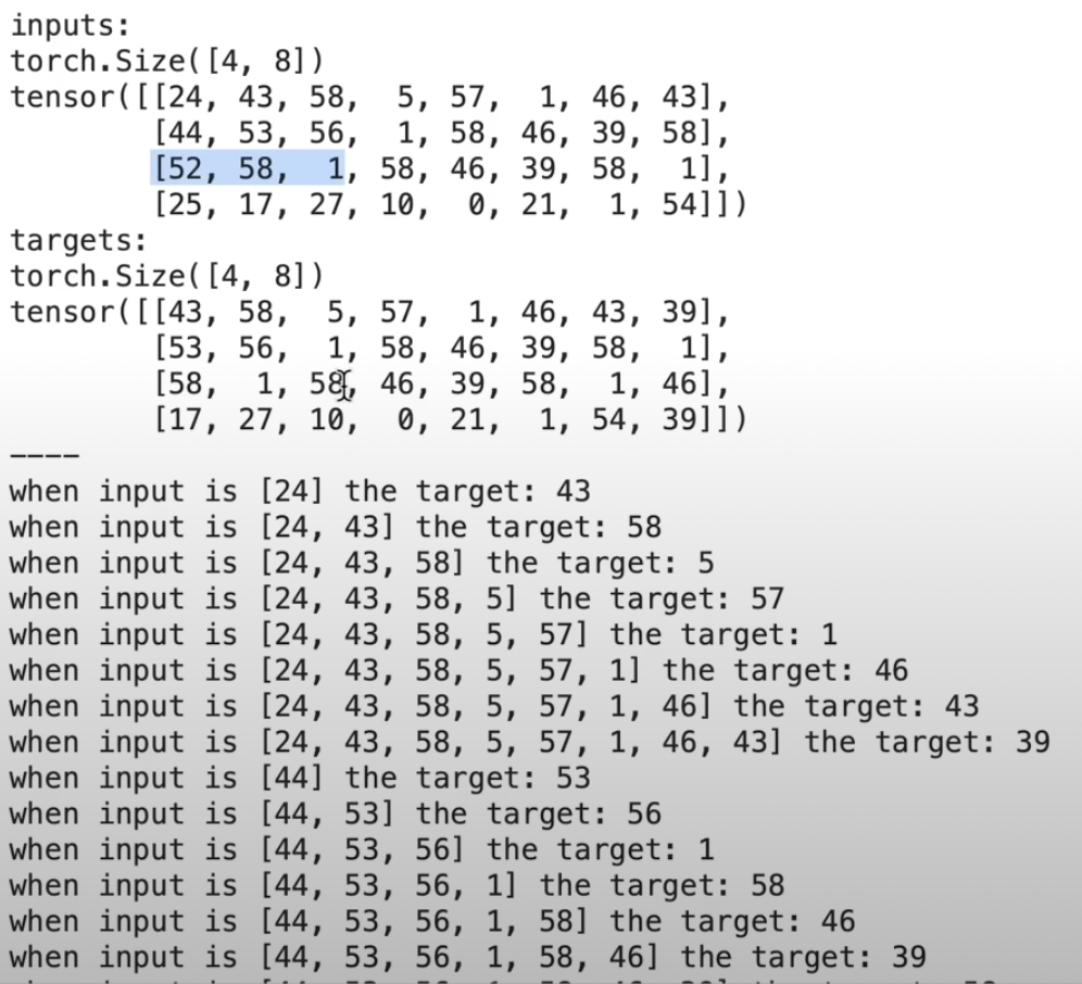
When we train the transformer, we train random little chunks at a time and the maximum length here will be called block size(a.k.a context length). When we think of language, the length increases with time so this can also be thought of as the time dimension.
For example when we have 9 elements in a list, we have 8 examples of dependencies that can be used to predict the next input.
1
tensor([18, 47, 56, 57, 58, 1, 15, 47, 58])
This will make it more efficient for us as we can start sampling generation later on with context as little as of one word. After block size, we will need to truncate for transformers can not deal large sizes of data.
Batch Size
On another note, we also care about batch dimensions. When we have multiple patches of sequences, how are we going to parallelize these? For the training efficiency of GPUs we stack them to a single tensor but in the training phase, it does not affect each other.
The tensors for our inputs and targets are seperately defined. You can see that both have the shape of batch size * block size - 4 * 8 in our case. This way for each batch we can generate sequences of 8 blocks and the 4 independent batches are sent to traverse through our model.
Bigram Model
The model will refer to the embedding table to find the corresponding row to the given index(word).
This embedding table will take the shape of (B, T, C) which denotes B: batch size, T: time(block size) and C: channels, meaning vocab size.
However the results from the bigram model won’t be stellar. It’s a simple one, so what do you expect? There’s definitely room to improve.
Past context
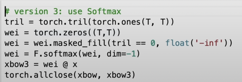
Now we want the tokens in a single batch to interact with each other but in a unidirectional way, from the left to the right. So we take the average of the preceding components.
The weights for the embedding matrix in the bigram model is (T, T) while the input will be (B, T, C). As the dimensions do not match for matrix multiplication, torch will add a batch dimension at the top hence (B, T, T) @ (B, T , C) = (B, T, C)
Tril will take the lower triangle of the matrix which is important for us because we only take information into account that travels to the right.
Now we will also run the weights through the softmax. If you think about the nature of softmax functions, the negative infinity will mask the upper triangle as the exponential in the softmax will return values to 0.
Position Embeddings
We also encode the position embeddings alongside the token embeddings. This will become useful for self-attention heads.
Self-attention
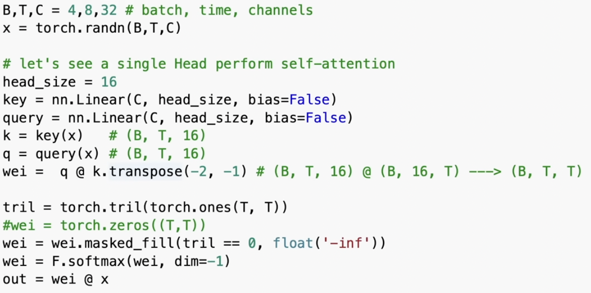
Now we include the data context into our weights using self-attention. Every single token will emit a query and a key.
Query: What am I looking for?
Key: What do I contain?
And the dot product of these two elements become weights. If the two align, it will result in a high value. The queries here are still indepedent of each other but the dot product between the queries and keys will render weights to be data-dependent.
Now we introduce a new variable, “value” which is just x propagated through a linear layer. The output will be the dotproduct of weights and values.
So the queries will specify what they are looking for: which position it is in, if it’s looking for a vowel after a consonant or not. And the key will tell you the answers to it. These two combined, will tell you the affinity of these interactions. Now the value will take these weights and be added into the output. “Assess how important you think I am and include me!”
Notes
- Self-attention is a communication mechanism and can be applied to any arbitrary directional graph.
- There is no notion of space, so you need positional encodings. Meanwhile, CNNs do provide an idea of positions.
- All examples in the batch dimension are independent.
- If you are doing sentiment analysis, you might do away with tril and let all the nodes communicate with each other.
- Cross-attention: Keys, queries and values don’t need to come from the same source. Keys and values can be from seperate sources that we would like to pool attention from.
- Since weights are fed into softamx, it’s important for them to be fairly diffused - that is with fixed variance. If the values are very extreme positive & negative values, softmax will converge to one-hot vectors. We can implement this by dividing with the root of head size.
Multi-headed Self-attention
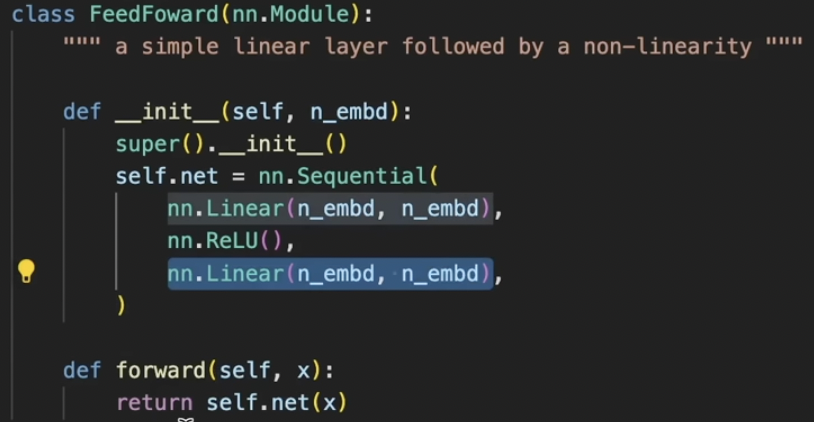
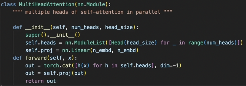
Applying multi heads and concatenate them, similar to group convolutions. After the attention head, the model needs time to process the data it was given. This is implemented through feed forward which consists of a linear layer and relu. This happens per node and therefore is independent.
Now we need to intersperse the communication with the computation. So it groups them and communicates them. To make things work channel-wise, we set head size to the number of embeddings divided by number of heads.
Skip Connections
To maintain the connections whilst depth, we use skip connections. The residual pathway can be forked away from. While backpropagation, it travels through back equally for addittions, so the gradients will make it all the way back from the supervision to the input, unimpeded.
In the beginning, it’s almost as if it’s not there but with optimization, they came online overtime and start to contribute.
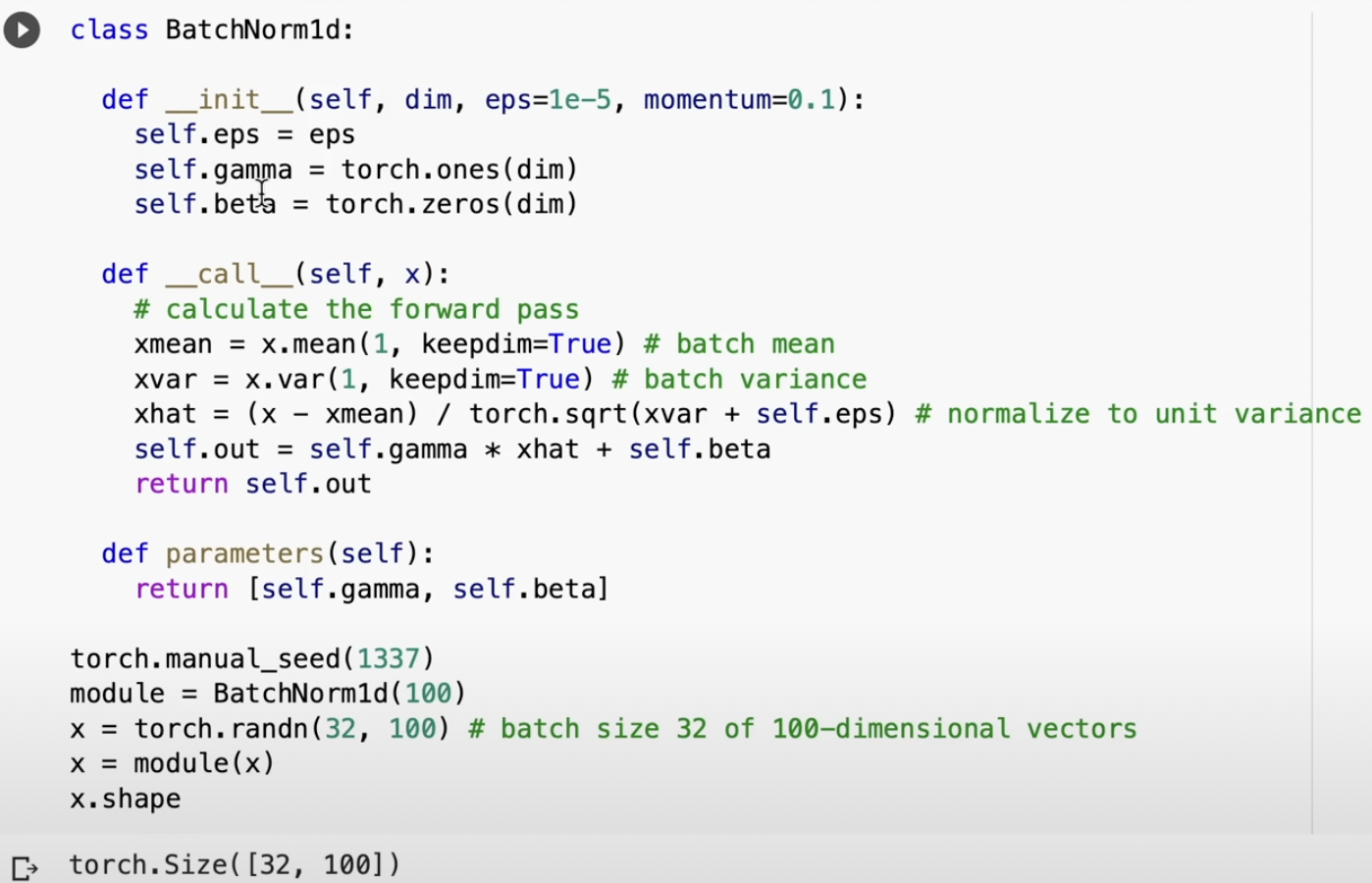
LayerNorm
Normalizes the rows instead of the columns. They will have unit Gaussian.
Dropouts
Every forward/backward path, it shuts off some subset of neurons, randomly drops them to 0 and train without them, so it trains an ensemble of subnetworks. If we scale up the model, it will help prevent overfitting.

